Searching Internet 🌐

Unfortunately, Google Sheets does not support freezing non-adjacent columns, such as columns A and Z. The freeze functionality allows you to only freeze contiguous columns or rows. This means that if you want to keep certain columns visible while scrolling, you must select a continuous range of columns rather than skipping columns in between.

To freeze columns in Google Sheets, you can follow these general steps:

1. Open Your Spreadsheet: Start by accessing your Google Sheets document.

2. Select a Column: Click on the letter header of the column that is immediately to the right of the last column you want to freeze (for example, if you want to freeze column A, click on the header of column B).

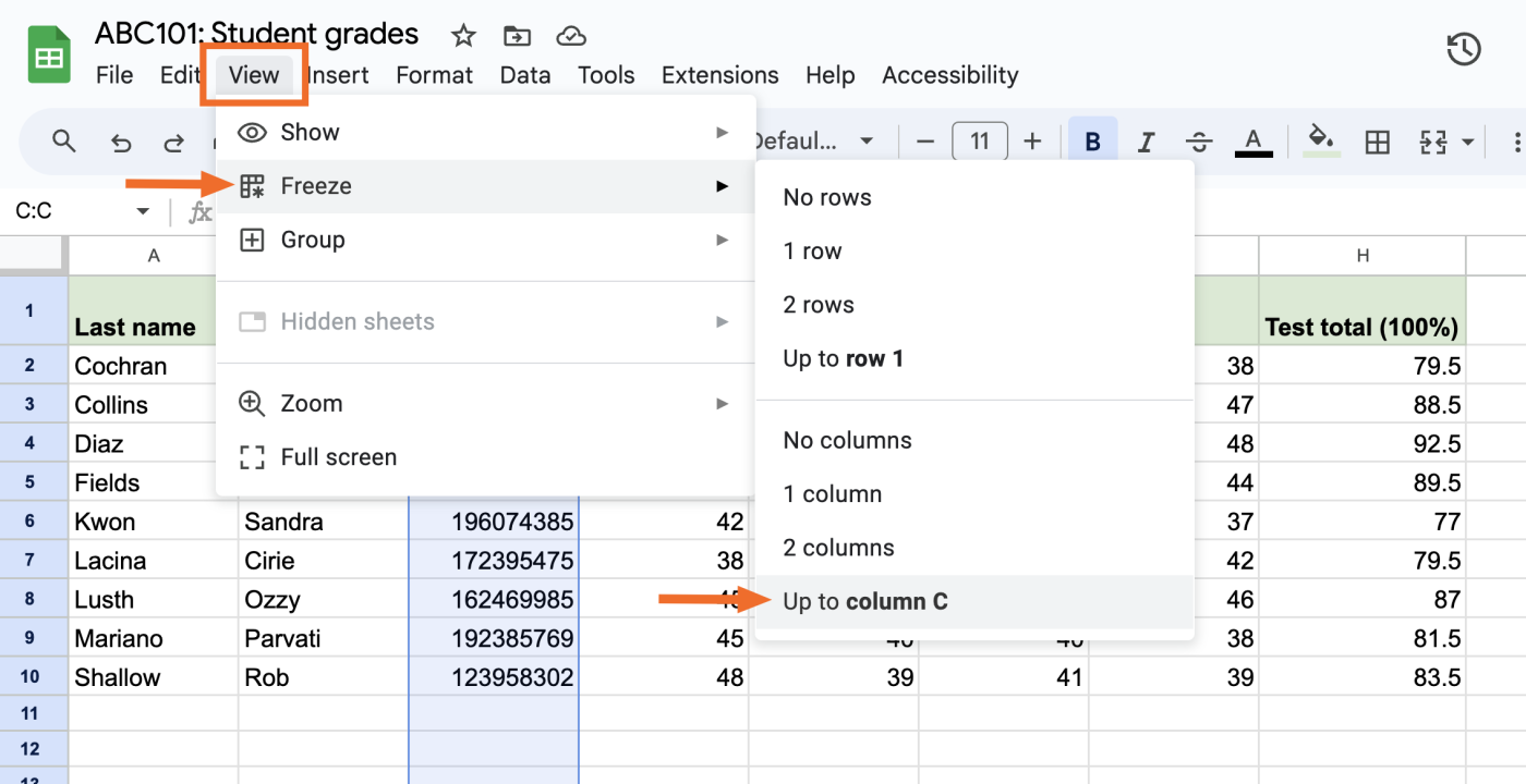
3. Access the View Menu: In the top menu, click on "View".

4. Choose Freeze Option: Hover over the "Freeze" option in the dropdown menu and select "1 column", "2 columns", or “Up to current column”, depending on how many you want to freeze.

For further information, you might find the official Google Help page useful, which explains how to freeze rows and columns here. Additionally, you can explore community discussions and examples in forums like Reddit for more context on handling data in Google Sheets.

In conclusion, if you need to keep both column A and column Z visible, you’ll have to find an alternative approach, such as arranging your spreadsheet differently or using a filter to manage your data effectively, since the functionality to freeze non-adjacent columns is not available.

Sources

Freeze, group, hide, or merge rows & columns - Google HelpCan't Freeze Vertical Columns in Sheets - Google HelpFreezing Multiple Nonconsecutive Columns in ExcelHow to freeze rows & columns (& How to unfreeze) in Google SheetsExcel 2010: "freeze" multiple, non-adjacent columns? - ProZ.comHow to Make Google Sheets Longer - Bricks AIHow to freeze rows then sort : r/googlesheets - Reddit

Related Questions

How do I freeze specific columns in Google Sheets?

How to select two columns that aren t next to each other in Google Sheets?

Why can't I freeze more than two columns in Google Sheets?

How do I lock certain columns in Google Sheets?